ABCD Matrices

The ABCD or ray-matrix formalism is used in the paraxial approximation of geometrical optics. A ray is characterised by its lateral position r relative to the central axis of the system, and the slope r'.

We can then define a 2 x 2 matrix for an optic or a set of optics that maps the incident r, r' to new values according to

LaserCanvas uses the reduced-angle convention described in A.E. Siegman, Lasers, University Science Books (1986). In this convention, the second element of the [r, r'] vector is not the geometric divergence angle, but the effective divergence reduced by refraction. The resulting ABCD matrices have unit determinant.

The ABCD matrices as used by LaserCanvas are listed in the following table.


Element	Parameters	Sagittal	Tangential

Space	Distance L Refractive index n
Lens	Focal length f
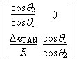
Mirror	Radius Curvature R (Concave: R > 0) Incidence angle
Curved dielectric	n₁sin₁ =n₂sin₂ n_SAG = n₂cos₂ - n₁cos₁ n_TAN =

Stability Parameter

For a resonator, the system stability can be calculated from the trace of the round-trip matrix M by

For stable resonators, |g| < 1. The stability parameter gives some indication of the robustness of the resonant mode against slight changes in the cavity configuration.

Internal Representation

The ABCD matrices are not explicitly stored. They are calculated whenever necessary from the optic properties. Since many of the optics' properties can be defined using equations, the ABCD matrices are, in general, not constant.

For the resonant and propagating mode calculations, the ABCD matrices are represented in a custom 4-element class using IEEE double precision. The matrix pre-multiplication used in resonator calculations is explicitly expanded by element.